For part 1, see here.
Overview of the software components
All the software written for this project is in Python. I’m not an expert python programmer, far from it but the huge number of available libraries and the fact that I can make some sense of it all without having spent a lifetime in Python made this a fairly obvious choice. There is a python distribution called Anaconda which takes the sting out of maintaining a working python setup. Python really sucks at this, it is quite hard to resolve all the interdependencies and version issues, using ‘pip’ and the various ways in which you can set up a virtual environment is a complete nightmare once things get over a certain complexity level. Anaconda makes that all managable and it gets top marks from me for that.
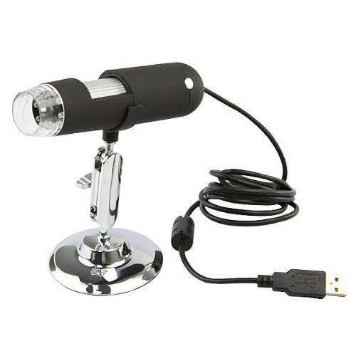
The Lego sorter software consists of several main components, there is the frame grabber which takes images from the camera:
Scanner / Stitcher
Then, after the grabber has done it’s work it sends the image to the stitcher which does two things: the first thing it does is determine how much the belt with the parts on it has moved since the previoue frame (that’s the function of that wavy line in the videos in part 1, that wavy line helps to keep track of the belt position even when there are no parts on the belt), and then it will update an in-memory image with the newly scanned bit of what’s under the camera. Whenever there is a vertical break between parts the stitched part gets cut and the newly scanned part gets sent on.
All this is done using OpenCV,
After the scanner/stitcher has done its job a part image looks like this:
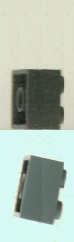
Stitching takes care of the situation where a part is longer than what fits under the camera in one go.
Parts Classification
This is where things get interesting. So, I’ve built this part several times now, to considerably annoyance.
OpenCV primitives
The first time I was just using OpenCV primitives, especially contour matching and circle detection. Between those two it was possible to do a reasonably accurate recognition of parts as long as there were not too many different kinds of parts. This, together with some simple meta data (l, w, h of the part) can tell the difference between all the basic lego bricks, but not much more than that.
Bayes
So, back to the drawing board: enter Bayes. Bayes classifiers are fairly well understood, you basically engineer a bunch of features, build detectors for those, create a test-set to verify that your detector works as advertised and you try to crank up the discriminating power of those features as much as you can. This you then run over as large a set of test images as you can to determine the ‘priors’ that will form the basis for the relative weighing of each feature as it is detected to be ‘true’ (feature is present) or ‘false’ (feature is not present). I used this to make a classifier based on the following features:
- cross (two lines meeting somewhere in the middle)
- circle (the part contains a circle larger than a stud)
- edge_studs (studs visible edge-on)
- full (the part occupies a large fraction of its outer perimeter)
- height
- holes (there are holes in the part)
- holethrough (there are holes all the way through the part)
- length
- plate (the part is roughly a plate high)
- rect (the part is rectangular)
- slope (the part has a sloped portion)
- skinny (the part occupies a small fraction of its outer perimeter)
- square (the part is roughly square)
- studs (the part has studs visible)
- trans (the part is transparent)
- volume (the volume of the part in cubic mm)
- wedge (the part has a wedge shape)
- width
And possibly others… This took quite a while. It may seem trivial to build a ‘studs detector’ but that’s not so simple. You have to keep in mind that the studs could be in any orientation, that there are many bits that look like studs but really aren’t and that the part could be upside-down or facing away from the camera. Similar problems with just about every feature so you end up tweaking a lot to get to acceptable performance for individual features. But once you have all that working you get a reasonable classifier for a much larger spectrum of parts.
Even so, this is far from perfect: it is slow, with every category you add you’re going to be doing more work in order to figure out which category a part is. The ‘best match’ can come from a library of parts which itself is growing so there is a nice geometrical element to the amount of computer time spent. Accuracy was quite impressive but in the end I abandoned this approach because of the speed (it could not keep up with the machine) and changed to the next promising candidate, an elimination based system.
Elimination
The elimination system used the same criteria as the ones listed before. Sorting the properties in decreasing order of effectiveness allowed a very rapid elimination of non-candidates, and so the remainder could be processed quite efficiently. This was the first time the software was able to keep up with the machine running full-speed.
There are a couple of problems with this approach: once something is eliminated, it won’t be back, even if it was the right part after all. The fact that it is a rather ‘binary’ approach really limits the accuracy, so you’d need a huge set of data to make this work, and that would probably reduce the overall effectiveness quite a bit.
It also ends up quite frequently eliminating all the candidates, which doesn’t help at all. So, accuracy wasn’t fantastic and fixing the accuracy would likely undo most of the speed gains.
Tree based classification
This was an interesting idea. I made a little tree along the lines of the Animal Guessing Game. Every time you add a new item to the tree it will figure out which of the features are different and it will then split the node at which the last common ancestor was found to accomodate the new part. This had some significant advantages over the elimination method: the first is that you can have a part in multiple spots in the tree which really helps accuracy. The second is that it is lightning fast compared to all the previous methods.
But it still has a significant drawback: you need to manually create all the features first and that gets really tedious, assuming you can even find ‘clear’ enough features that you can write a straight up feature detector using nothing but OpenCV primitives. And that can get challenging fast, especially because python is a rather slow language and if your problem can’t be expressed in numpy or OpenCV library calls you’ll be looking at a huge speed penalty.
Machine Learning
Finally! So, after roughly 6 months of coding up features, writing tests and scanning parts I’d had enough. I realized that there is absolutely no way that I’ll be able to write a working classifier for the complete spectrum of parts that Lego offers and that was a real let-down.
So, I decided to bite the bullet and get into machine learning in a more serious manner. For weeks I read papers, studied all kinds of interesting bits and pieces regarding Neural Networks.
I had already played with when they first became popular in the 1980’s after reading a very interesting book on a related subject. I used some of the ideas in the book to rescue a project that was due in a couple of days where someone had managed to drop a coin into the only prototype of a Novix based Forth computer that was supposed to be used for a demonstration of automatic license plate recognition. So, I hacked together a bit of C code with some DSP32 code to go with it and made the demo work, and promptly forgot about the whole thing.
A lot has happened in the land of Neural Networks since then, the most amazing thing is that the field almost died and now it is going through this incredible rennaisance powering all kinds of real world solutions. We owe all that to a guy called Geoffrey Hinton who just simply did not give up and turned the world of image classification upside down by winning a competition in a most unusual manner.
After that it seemed as if a dam had been broken, and one academic record after another was beaten with huge strides forward in accuracy for tasks that historically had been very hard for computers (vision, speech recognition, natural language processing).
So, lots of studying later I had settled on using TensorFlow, a huge library of very high quality produced by the Google Brain Team, where some of the smartest people in this field in the world are collaborating. Google has made the library open-source and it is now the foundation of lots of machine learning projects. There is a steep learning curve though, and for quite a while I found myself stuck on figuring out how to proceed best.
And then several things happened in a very short time: about two months ago HN user greenpizza13 pointed me at Keras, rather than going the long way around and using TensorFlow directly (and Anaconda actually does save you from having to build TensorFlow). And this in turn led me to Jeremy Howard and Rachel Thomas’ excellent starter course on machine learning.
Within hours (yes, you read that well) I had surpassed all of the results that I had managed to painfully scrounge together feature-by-feature over the preceding months, and within several days I had the sorter working in real time for the first time with more than a few classes of parts. To really appreciate this a bit more: approximately 2000 lines of feature detection code, another 2000 or so of tests and glue was replaced by less than 200 lines of (quite readable) Keras code, both training and inference.
The speed difference and ease of coding was absolutely incredible compared to the hand-coded features. While not quite as fast as the tree mechanism accuracy was much higher and the ability to generalize the approach to many more classes without writing code for more features made for a much more predictable path.
The hard challenge to deal with next was to get a training set large enough to make working with 1000+ classes possible. At first this seemed like an insurmountable problem. I could not figure out how to make enough images and to label them by hand in acceptable time, even the most optimistic calculations had me working for 6 months or longer full-time in order to make a data set that would allow the machine to work with many classes of parts rather than just a couple.
In the end the solution was staring me in the face for at least a week before I finally clued in: it doesn’t matter. All that matters is that the machine labels its own images most of the time and then all I need to do is correct its mistakes. As it gets better there will be fewer mistakes. This very rapidly expanded the number of training images. The first day I managed to hand-label about 500 parts. The next day the machine added 2000 more, with about half of those labeled wrong. The resulting 2500 parts where the basis for the next round of training 3 days later, which resulted in 4000 more parts, 90% of which were labeled right! So I only had to correct some 400 parts, rinse, repeat… So, by the end of two weeks there was a dataset of 20K images, all labeled correctly.
This is far from enough, some classes are severely under-represented so I need to increase the number of images for those, perhaps I’ll just run a single batch consisting of nothing but those parts through the machine. No need for corrections, they’ll all be labeled identically.
I’ve had lots of help in the last week since I wrote the original post, but I’d like to call out two people by name because they’ve been instrumental in improving the software and increasing my knowledge, the first is Jeremy Howard, who has gone over and beyond the call of duty to fill in the gaps in my knowledge, without his course I would have never gotten off the ground in the first place, and second Francois Chollet, the maker of Keras who has been extremely helpful in providing a custom version of his Xception model to help speed up training.
Right now training speed is the bottle-neck, and even though my Nvidia GPU is fast it is not nearly as fast as I would like it to be. It takes a few days to generate a new net from scratch but I simply don’t think it is responsible to splurge on a 4 GPU machine in order to make this project go faster. Patience is not exactly my virtue but it looks as though I’ll have to get more of it. At some point all the software and data will be made open source, but I still have a long way to go before it is ready for that.
Once the software is able to reliably classify the bulk of the parts I’ll be pusing through the huge mountain of bricks, and after that I’ll start selling off the result, both sorted parts as well as old sets.
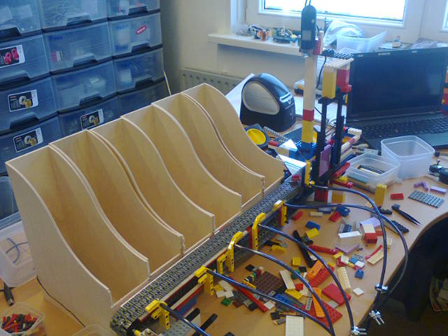
Finally, to close off this post, an image of the very first proof-of-concept, entirely made out of Lego: